The so-called Conditional Formatting, is a practical feature with which Excel can set the format of the corresponding data. One example is that when you want to highlight some specified data in a spreadsheet, you can use Conditional Formatting to shade them automatically avoiding a lot of manual operations.
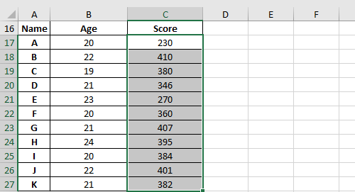
First, select the range of cells you want apply the conditional format to.
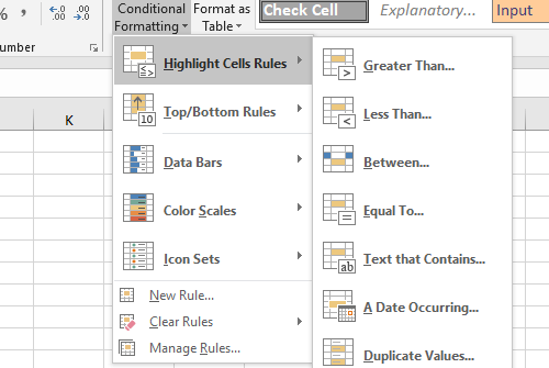
Find Conditional Formatting in Home tab.

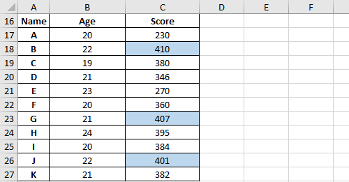
There are many existing rules in the drop-down menu you can directly choose and use. In my case, I want to shade all the data larger than 400 in the Score column of my table. So choose Greater Than… in Highlight Cell Rules.
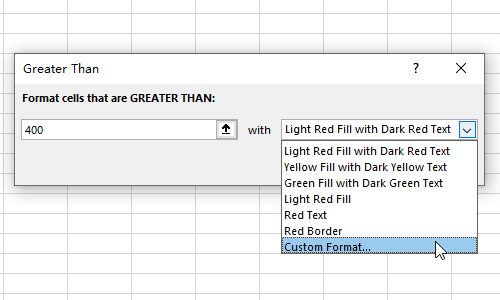
Type the number 400 in the text box and choose a format color. If you don’t like these color schemes in the drop-down list, hit Custom Format…
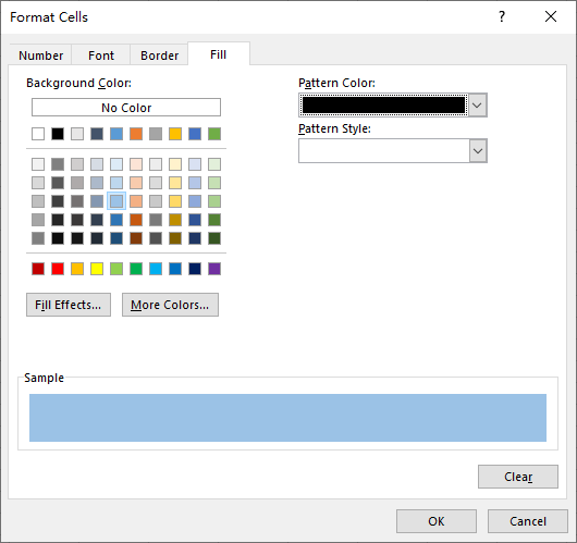
Switch to Fill tab and select the Background Color and Pattern Color you like. Click OK to confirm the settings and hit OK again in Greater Than window.
Now the format you customized is applied to all the data greater than 400 in Score column.
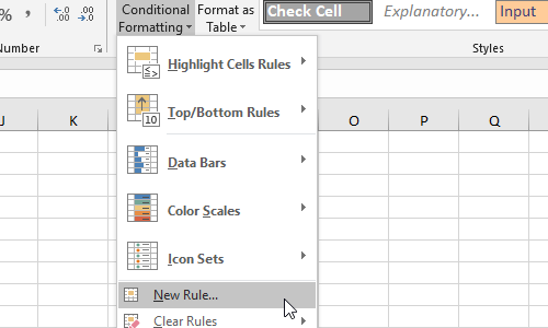
If you’re not satisfied with the existing rules, you can create a new one by clicking New Rule… in Conditional Formatting.
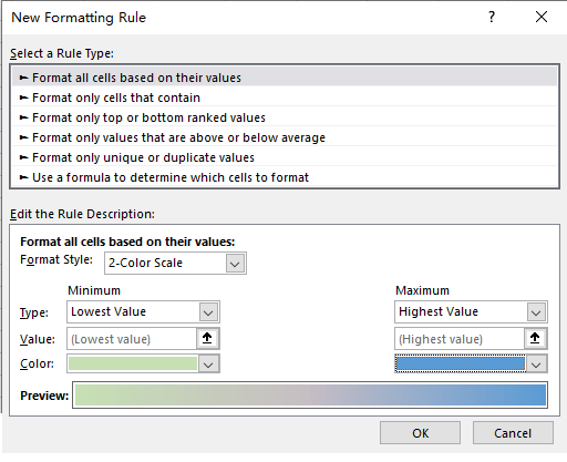
There are many rule types in the list. Take the first one as an example, you can set a color for the Lowest Value and another color for the Highest Value. It will create a set of gradient color for you. Click OK to apply it to your worksheet.
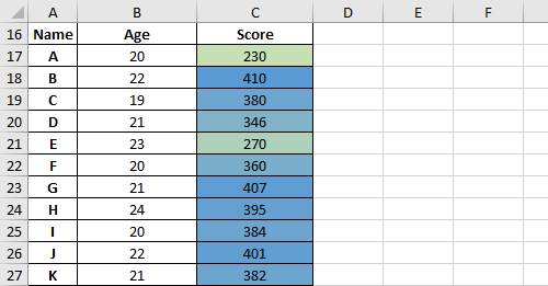
Then all the selected data will be shaded with the color from green to blue in ascending order.
This is just a quick start guide for Conditional Formatting. There are much more practical cases you can make use of it and improve your spreadsheet skillfully.

Hi there colleagues, good paragraph and good arguments commented at this place, I am really enjoying by
these.