VLOOKUP is a very useful Excel function which can easily search through a column and find the corresponding data. For example, you can search for the score of a student in class quickly according to his or her name.
The basic formula for VLOOKUP is:
=VLOOKUP (lookup_value,table_array,col_index_num,range_lookup)
“lookup_value” refers to the keyword for searching;
“table_array” is the range of matching object;
“col_index_num” indicates the column number of the result;
“range_lookup” refers to the matching mode, which contains two options: “0” for accurate matching and “1” for fuzzy matching.
Assuming there’s a very long list of record in the table below, now I want to find the score of someone, how can I do it with VLOOKUP function?
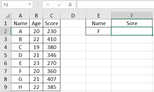
First, input the formula in the cell to output the search result which should be F2 in my case. So I click F2 and hit the small icon of “fx” above the table.

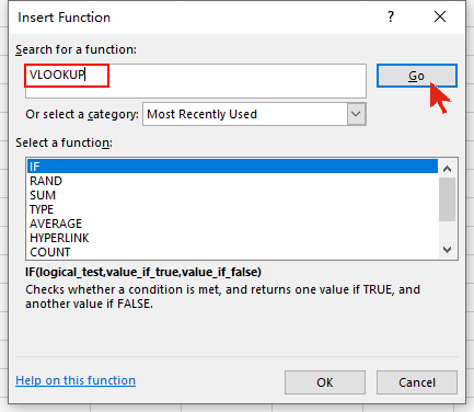
Type “VLOOKUP” directly in the textbox of Search for a function and hit Go.
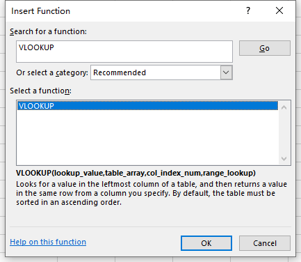
Click VLOOKUP in the section of Select a function and click OK to insert the formula.
Then you can input the value of each factor of the formula. For example, I want find the score of F in the table, so the Lookup_value should be “F“. And his score is in the third column, so the Col_index_num is doubtlessly “3“. To find an accurate result, I can set the Range_lookup as “0“.
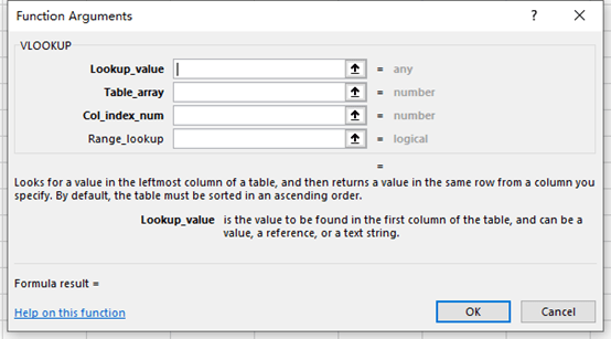
As for the Table_array, a convenient way is clicking the small arrow on the right of the textbox, then hold and drag the left mouse to select all the cells in the table. The range of table will be inserted to the textbox accordingly. Click that small arrow again, we can get back to Function Arguments window and continue editing.
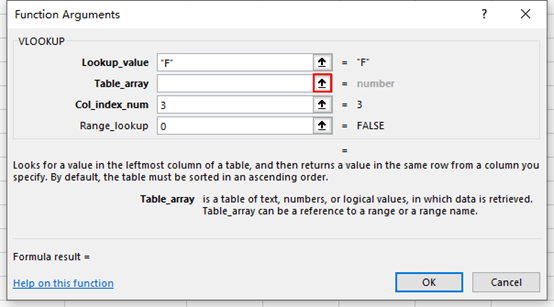
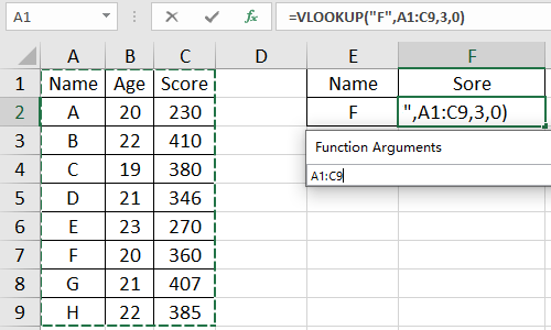
Now all the textbox have been filled up, you can see the formula in F2 is also completed at the same time. In fact, you can directly complete and input the formula after being familiar with the function.
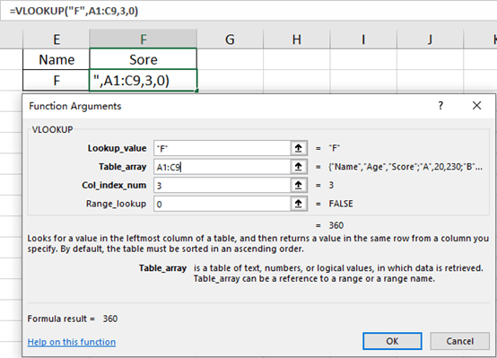
Click OK to close the Function Arguments window. VLOOKUP function has found the data I’m looking for in F2.
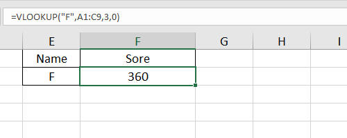
This is the basic application of VLOOKUP function in Excel. In practical work, there are much more usages of it for sure. I’ll probably continue this topic in future posts.

Like!! Great article post.Really thank you! Really Cool.