If you’ve made a pie chart in Excel, you can apply any color or style you like to it easily. But if you’re not satisfied with the location of these slices, how can you rotate the pie chart to finally meet your need?
Look at this chart below, the blue slice of A is on the upper right of the pie. But personally I want it to be on the left. The detailed steps are as below.

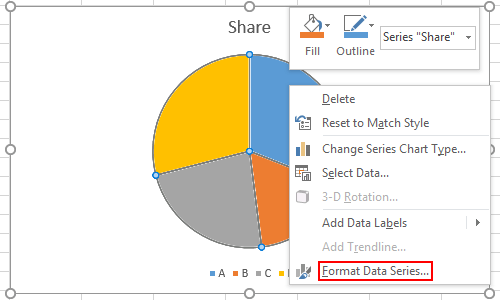
1. First, double-click the pie chart to enable Format Data Series… panel on the right of Excel spreadsheet, or you can right-click it and choose Format Data Series… in the menu.
Please note that you should click exactly on the pie chart instead of the blank background of the chart area.
2. The Format Data Series panel will show on the right of the page.
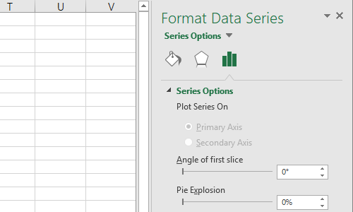
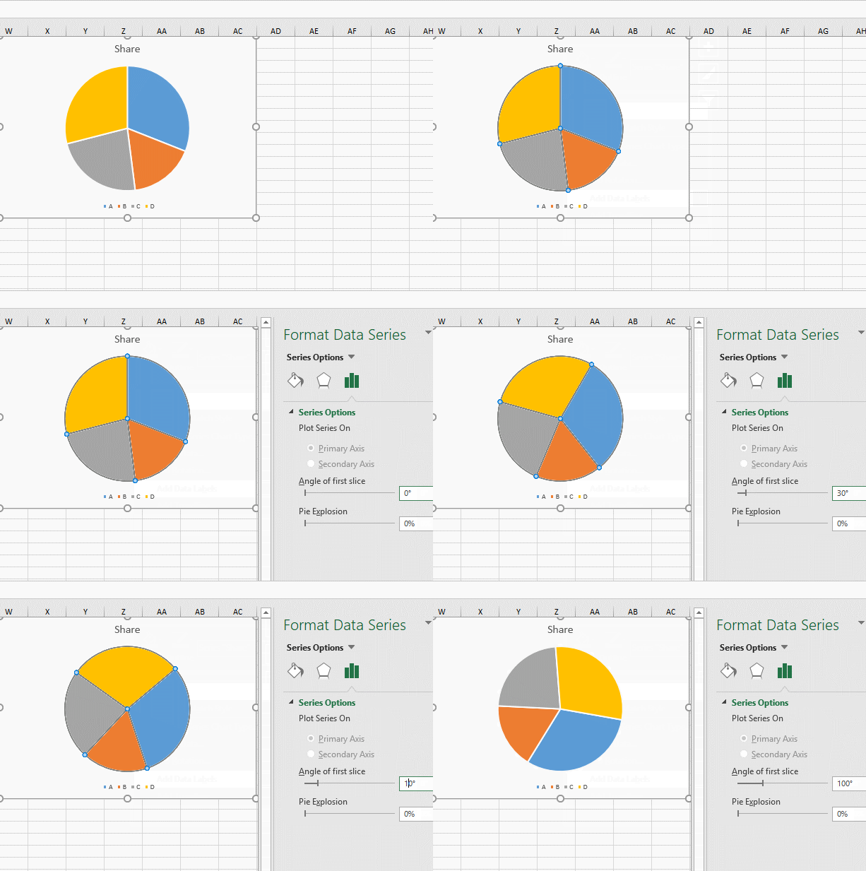
3. Switch to Series Options (the icon of histogram) and you can adjust the Angle of first slice here. Change the value in the textbox, the pie chart will rotate accordingly.
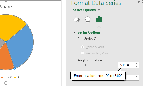
4. You can input different angles to rotate the slices till it finally meets your need.
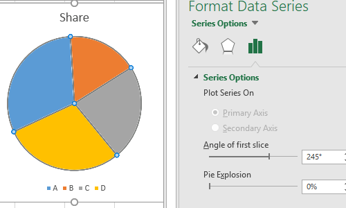
The complete process of rotating Excel pie charts is as below.

Leave a Reply